Supersonic Propulsion - Design Research Projects

The two papers included in this post are from a course called “Rocket Science” which was essentially an introduction to compressible flow and supersonic propulsion.

The first paper is about optimizing a body to minimize pressure and viscous drag. It is relatively brief, but I think it is a good demonstration of formulating an approach and reaching a reasonable answer for a generic problem.

Pressure Drag Optimization

📄View PDF in dedicated tab

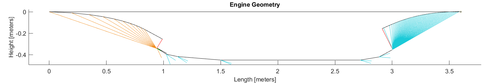
The second paper is a group project describing the design of a ramjet engine. I did a lot of the coding and CAD, and I am pretty proud of the product that we came up with given what we knew back then. Ignoring the caveat that the geometry is all two-dimensional, the inlet design almost makes sense, other than the fact that the turning angle is very high. The expanding nozzle is also reasonable given that it was designed using MOC. The cowl is way too thin to take any load. We won’t even get into the combustor since I still don’t know how that works. Enjoy JP’s pretty CFD plots!

Full Engine Design

📄View PDF in dedicated tab

Fuselage Oblique and Expansion Waves

Engine Design Code in MATLAB

    %%%%%%%%%%%%%%%%%%%%%%%%%%%%%%%%%%%%%%%%%%%%%%%%%%%%%%%%%%%%%%%%%
    %                 Final Project - Ramjet Engine                 %
    %                           5/10/2024                           %
    %%%%%%%%%%%%%%%%%%%%%%%%%%%%%%%%%%%%%%%%%%%%%%%%%%%%%%%%%%%%%%%%%

    clc
    clear
    close all

    % This script is for calculating the engine design. Evaluation of the
    % design at all operating points is done in another script.

    % Full description of the model, assumptions, calculation approach, and
    % work done by each team member can be found detailed in our final report.

    %% Flags to enable certain portions of the code:
    PlotInlet_MaxM = 1; % Boolean for plotting the inlet at M1=3.25
    PlotInlet_MinM = 0; % Boolean for plotting the inlet at flow properties specified below
    PlotNozzle = 1; % Boolean for plotting the outlet

    %% Incoming Flow Properties
    M1 = 3.25;
    % Assumed pressure and temperature at 55,000 ft
    P1 = 9450; % Pa
    T1 = 216; % K
    gamma = 1.4;
    R_air = 287; % J/kg*K
    rho1 = P1/(R_air*T1); % kg/m^3
    u1 = M1*sqrt(gamma*R_air*T1);

    %% Inlet
    % The inlet ramp is designed at maximum operating Mach 3.25 to avoid
    % complications from the oblique shocks entering and causing distortion.
    Mach_max = 3.25;

    % Overall inlet geometry parameters
    theta_total = 30; % Degrees, total turn angle
    n_sections = 10; % Number of turn sections
    theta_increment = theta_total/n_sections;

    % Calculate properties along each section of inlet
    M_inlet_design = zeros(n_sections+1,1); beta_design = zeros(n_sections,1); % Allocate Memory
    M_inlet_design(1) = Mach_max; % Assign initial value
    for i = 1:n_sections
        % Call ObliqueShock function repeatedly
        [M_inlet_design(i+1), ~, ~, beta_design(i)] = ObliqueShock(M_inlet_design(i), gamma, theta_increment);
    end

    % Calculate section lengths such that all the waves intersect at a single point.
    [os_wavelength, section_lengths] = deal(zeros(n_sections,1)); % Allocate Memory
    % The following parameter is used to scale the entire engine. It is the
    % length of the first oblique shock wave up to the intersection point ahead
    % of the cowl:
    os_wavelength(1) = 1; % Meters

    for i = 2:n_sections
        % Calculate the lengths of each subsequent section using law of sines.
        section_lengths(i-1) = os_wavelength(i-1)*sind(beta_design(i)-beta_design(i-1)+theta_increment)/sind(180-beta_design(i));
        os_wavelength(i) = os_wavelength(i-1)*sind(beta_design(i-1)-theta_increment)/sind(180-beta_design(i));
    end

    % Calculate angles with respect to global coordinate system
    theta_sum = zeros(n_sections+1,1); beta_design_global = zeros(n_sections,1); % Allocate Memory
    for i = 1:n_sections
        theta_sum(i+1) = theta_sum(i) + theta_increment;
        beta_design_global(i) = beta_design(i) + theta_sum(i);
    end

    % Calculate inlet coordinates and shock intersection locations to double
    % check geometry.
    [x_inlet,y_inlet] = deal(zeros(n_sections+1,1)); % Allocate Memory
    [x_beta_design,y_beta_design] = deal(zeros(n_sections,1));
    for i = 1:n_sections
        x_inlet(i+1) = x_inlet(i) + section_lengths(i)*cosd(theta_sum(i+1));
        y_inlet(i+1) = y_inlet(i) - section_lengths(i)*sind(theta_sum(i+1));
        x_beta_design(i) = x_inlet(i) + os_wavelength(i)*cosd(beta_design_global(i));
        y_beta_design(i) = y_inlet(i) - os_wavelength(i)*sind(beta_design_global(i));
    end

    % We want 5% of the flow to be wasted at 3.25 mach as a safety margin.
    % Calculate the position of the cowl to satisfy this constraint.
    s_para = -tand(theta_total);
    s_perp = -1/s_para;
    x_ns_top = (y_beta_design(n_sections) - y_inlet(n_sections+1) + s_para*x_inlet(n_sections+1) - s_perp*x_beta_design(n_sections))/(s_para-s_perp);
    y_ns_top = s_para*(x_ns_top-x_inlet(n_sections+1))+y_inlet(n_sections+1);
    delta_x = x_beta_design(n_sections) - x_ns_top;
    delta_y = y_beta_design(n_sections) - y_ns_top;
    x_ns_cowl = 0.95*delta_x + x_ns_top;
    y_ns_cowl = 0.95*delta_y + y_ns_top;

    inlet_coordinates = [x_inlet y_inlet ; x_ns_top y_ns_top ; x_ns_cowl y_ns_cowl];

    %% Plot inlet at design condition M1=3.25
    if PlotInlet_MaxM == 1
        fig = figure;
        hold on
        % Inlet top geometry
        plot(x_inlet(1:n_sections),y_inlet(1:n_sections),'-xk')
        plot([x_inlet(n_sections) x_ns_top],[y_inlet(n_sections) y_ns_top],'-k')
        % Oblique shocks
        for i=1:n_sections
            plot([x_inlet(i) x_beta_design(i)],[y_inlet(i) y_beta_design(i)],Color='#F19024')
        end
        % Normal Shock
        plot([x_ns_top x_ns_cowl],[y_ns_top y_ns_cowl],'r')
        % Cowl point
        plot(x_ns_cowl,y_ns_cowl,'*b')
        %plot([x_ns_cowl+0.1*cosd(theta_total+15) x_ns_cowl x_ns_cowl+0.1*cosd(theta_total)],[y_ns_cowl-0.1*sind(theta_total+15) y_ns_cowl y_ns_cowl-0.1*sind(theta_total)],'-k')
        xlabel("Length [meters]")
        ylabel("Height [meters]")
        title("Inlet Geometry")
        fontsize(15,'points')

        % Size margins and plot for screen
        xmin = 0;
        xmax = x_ns_top;
        ymin = y_beta_design(n_sections);
        ymax = 0;
        dx = xmax-xmin;
        dy = ymax-ymin;
        ar = dy/dx;
        cushion = 0.05;
        xlim([xmin - cushion*dx xmax + cushion*dx])
        ylim([ymin - cushion*dy ymax + cushion*dy])
        screenx = 1920;
        screeny = 1080;
        fig.Position = [0 0.5*(screeny-screenx*ar) screenx screenx*ar];
    end

    %% Inlet at set Mach Number
    % Now that the above code has been ran for 3.25 mach, the geometry can be
    % locked in and we can determine the oblique shock pattern for other mach
    % numbers.
    % Calculate properties along each section of inlet
    [M_inlet,P_inlet,T_inlet] = deal(zeros(n_sections+1,1)); beta = zeros(n_sections,1); % Allocate Memory
    M_inlet(1) = M1; P_inlet(1) = P1; T_inlet(1) = T1; % Assign initial values
    for i = 1:n_sections
        % Call ObliqueShock function repeatedly
        [M_inlet(i+1), P_ratio, T_ratio, beta(i)] = ObliqueShock(M_inlet(i), gamma, theta_increment);
        P_inlet(i+1) = P_ratio*P_inlet(i); T_inlet(i+1) = T_ratio*T_inlet(i);
    end

    % Calculate angles with respect to global coordinate system
    beta_global = zeros(n_sections,1); % Allocate Memory
    for i = 1:n_sections
        beta_global(i) = beta(i) + theta_sum(i);
    end

    % Calculate oblique shock lines up until the cowl y coordinate.
    [x_beta,y_beta] = deal(zeros(n_sections,1));
    for i = 1:n_sections
        slope = -tand(beta_global(i));
        x_beta(i) = x_inlet(i) + (y_ns_cowl-0.1-y_inlet(i))/slope;
        y_beta(i) = y_ns_cowl-0.1;
    end

    % Calculate line from last shock intersection and make sure the flow coming
    % into the throat is uniform.
    s1 = -tand(beta_global(n_sections-1));
    s2 = -tand(beta_global(n_sections));
    x_lastshockint = (y_inlet(n_sections)-y_inlet(n_sections-1)-s2*x_inlet(n_sections)+s1*x_inlet(n_sections-1))/(s1-s2);
    y_lastshockint = s2*(x_lastshockint - x_inlet(n_sections)) + y_inlet(n_sections);
    x_dodgecowl = x_lastshockint + 0.05*cosd(theta_total);
    y_dodgecowl = y_lastshockint - 0.05*sind(theta_total);

    %% Plot inlet at Mach specified in Incoming flow properties
    if PlotInlet_MinM == 1
        fig = figure;
        hold on
        % Inlet top geometry
        plot(x_inlet(1:n_sections),y_inlet(1:n_sections),'-xk')
        plot([x_inlet(n_sections) x_ns_top],[y_inlet(n_sections) y_ns_top],'-k')
        % Oblique shocks
        for i=1:n_sections
            plot([x_inlet(i) x_beta(i)],[y_inlet(i) y_beta(i)],Color='#F19024')
        end
        % Normal Shock
        plot([x_ns_top x_ns_cowl],[y_ns_top y_ns_cowl],'r')
        % Cowl point
        plot(x_ns_cowl,y_ns_cowl,'*b')
        % Last disturbed flow approaching inlet
        plot([x_lastshockint x_dodgecowl],[y_lastshockint y_dodgecowl],'-g')
        %plot([x_ns_cowl+0.1*cosd(theta_total+15) x_ns_cowl x_ns_cowl+0.1*cosd(theta_total)],[y_ns_cowl-0.1*sind(theta_total+15) y_ns_cowl y_ns_cowl-0.1*sind(theta_total)],'-k')
        xlabel("Length [meters]")
        ylabel("Height [meters]")
        title("Inlet Geometry")
        fontsize(15,'points')

        % Size margins and plot for screen
        xmin = 0;
        xmax = x_ns_top;
        ymin = y_beta(n_sections);
        ymax = 0;
        dx = xmax-xmin;
        dy = ymax-ymin;
        ar = dy/dx;
        cushion = 0.05;
        xlim([xmin - cushion*dx xmax + cushion*dx])
        ylim([ymin - cushion*dy ymax + cushion*dy])
        screenx = 1920;
        screeny = 1080;
        fig.Position = [0 0.5*(screeny-screenx*ar) screenx screenx*ar];
    end

    %% Cowl (Normal Shock)
    Cowl_Area = 0.95*sqrt(delta_x^2 + delta_y^2); %m Area per unit depth at normal shock
    M2 = M_inlet(n_sections+1);
    P2 = P_inlet(n_sections+1);
    T2 = T_inlet(n_sections+1);
    m_dot_2 = P2*M2*Cowl_Area*sqrt(gamma/(R_air*T2)); %kg/s/m Mass flow per unit depth
    m_dot_air = m_dot_2;

    % Normal Shock Relations to determine state after normal shock
    g = gamma;
    M2_p = sqrt((1 + 0.5*(g-1)*M2^2)/(g*M2^2 - 0.5*(g-1)));
    P2_p = P2*(1 + (2*g*(M2^2 - 1))/(g+1));
    T2_p = T2*(1 + (2*g*(M2^2 - 1))/(g+1))*((2 + (g-1)*M2^2)/((g+1)*M2^2));
    m_dot_2_p = P2_p*M2_p*Cowl_Area*sqrt(gamma/(R_air*T2_p));

    % Stagnation state
    T0_2_p = T2_p*(1 + 0.5*(g-1)*M2_p^2);
    P0_2_p = P2_p*(1 + 0.5*(g-1)*M2_p^2)^(g/(g-1));

    %% Quasi-1D expansion of subsonic flow
    % A/A* at 2 after the normal shock:
    A_star_ratio_2p = (1/M2_p)*((2+(g-1)*M2_p^2)/(g+1))^(0.5*(g+1)/(g-1));
    A_star_sec1 = Cowl_Area/A_star_ratio_2p;

    % We can change this variable to set the flow characteristics going into
    % the combustor.
    A3 = 0.4; % Meters, area per unit depth before the flameholder
    A_star_ratio_3 = A3/A_star_sec1;

    % Use Newton's method to find Mach number at 3
    M_search = 0.5; % Start search on the correct side of the curve
    M_temp = 0; % Placeholder value
    delta = 1; % Placeholder value for step difference
    while delta > 0.0000000001
        innerterm = (2+(g-1)*M_search^2)/(g+1); % Base term that gets reused
        Astarfunction = (M_search^-2) * innerterm^((g+1)/(g-1)) - A_star_ratio_3^2;
        dfdM = (2/M_search) * (innerterm)^(2/(g-1)) * (1 - innerterm/(M_search^2));
        M_temp = M_search - 0.01*Astarfunction/dfdM; 
        % Had to make the scaling small (0.01) to make sure it doesn't 
        % overshoot to the negative side of the function.
        delta = abs(M_temp-M_search);
        M_search = M_temp;
    end
    M3 = M_search;

    % Isentropic flow means stagnation state has not changed from 2p
    T3 = T0_2_p/(1 + 0.5*(g-1)*M3^2);
    P3 = P0_2_p/(1 + 0.5*(g-1)*M3^2)^(g/(g-1));
    u3 = M3*sqrt(gamma*R_air*T3);
    rho3 = P3/(R_air*T3);
    m_dot_3 = P3*M3*A3*sqrt(gamma/(R_air*T3));


    %% Flameholder
    % Adiabatic Pressure Drop
    P3_p = P3*(1-0.81*gamma*M3^2);
    T3_p = T3;
    A3_p = A3;
    rho3_p = P3_p/(R_air*T3_p);

    % Across the pressure drop, mass must be conserved
    u3_p = rho3*u3/rho3_p;
    M3_p = u3_p/sqrt(gamma*R_air*T3_p);
    m_dot_3_p = P3_p*M3_p*A3_p*sqrt(gamma/(R_air*T3_p));
    % Confirm adiabatic
    T0_3_p = T3_p*(1 + 0.5*(g-1)*M3_p^2);

    %% Combustor
    % Stoichiometric Ratio for H2 and Air
    % https://www1.eere.energy.gov/hydrogenandfuelcells/tech_validation/pdfs/fcm03r0.pdf
    fuel_air_massratio_stoic = 1/34.33;
    % Equivalence ratio, manage this so that we avoid unstart from too much
    % heating.
    phi = 1; % For M1=2.75, phi = 1. For any M1>2.75, phi will decrease to choke at nozzle throat.
    m_dot_fuel = m_dot_air * phi * fuel_air_massratio_stoic;
    Lfv_H2 = 120*10^6; % J/kg, Lower heating value of H2
    q_addn = Lfv_H2*m_dot_fuel/m_dot_air; % J/kg, Heat addition (per unit mass of air) due to fuel combustion

    % Find state after instantaneous heat addition
    [M4,P4,T4] = HeatAddition_1D(q_addn,M3_p,P3_p,T3_p,R_air,gamma);
    % Find "average" velocity, pressure, and stagnation temperature during heating
    u4 = M4*sqrt(g*R_air*T4);
    u_avg = 0.5*(u3_p+u4);
    P_avg = 0.5*(P3_p+P4);
    P0_4 = P4*(1 + 0.5*(g-1)*M4^2)^(g/(g-1));
    T0_3_p = T3_p*(1+0.5*(g-1)*M3^2);
    T0_4 = T4*(1+0.5*(g-1)*M4^2);
    T0_avg = 0.5*(T0_3_p+T0_4);
    % Calculate a few different combustion times based on different points in
    % the process to see how much they differ. All have units of seconds.
    tau_3 = 325*(P3_p/101325)^(-1.6)*exp(-0.8*T0_3_p/1000)*10^-6;
    tau_avg = 325*(P_avg/101325)^(-1.6)*exp(-0.8*T0_avg/1000)*10^-6;
    tau_4 = 325*(P4/101325)^(-1.6)*exp(-0.8*T0_4/1000)*10^-6;
    % Required length for full combustion
    L_required = u_avg*tau_avg; % meters

    A4 = A3_p;
    m_dot_4 = P4*M4*A4*sqrt(gamma/(R_air*T4));

    %% Quasi 1D Compression
    % A/A* at 4 after combustion:
    A_star_ratio_4 = (1/M4)*((2+(g-1)*M4^2)/(g+1))^(0.5*(g+1)/(g-1));
    % Throat State:
    A5 = A3/A_star_ratio_4;
    M5 = 1;
    T5 = T0_4/(1 + 0.5*(g-1)*M5^2);
    P5 = P0_4/(1 + 0.5*(g-1)*M5^2)^(g/(g-1));

    m_dot_5 = P5*M5*A5*sqrt(gamma/(R_air*T5));

    %% Nozzle Design
    % In order to get the aerodynamic sizing we want, we need to figure out the
    % shape of the nozzle that will achieve the desired expansion.
    P6 = 5*P1; % Pa, desired exit pressure
    M6 = sqrt((2/(g-1)) * ((1+0.5*(g-1)*M5^2)*(P5/P6)^((g-1)/g) - 1));
    T6 = T0_4/(1 + 0.5*(g-1)*M6^2);
    u6 = M6*sqrt(g*R_air*T6);
    rho6 = P6/(R_air*T6);

    % Required expansion wave theta to achieve this pressure change.
    theta_expansion = PrandtlMeyerD(M6, gamma) - PrandtlMeyerD(M5, gamma);
    mu6 = asind(1/M6);
    n_nz_sections = 500; % Number of rays (waves) to propogate
    turn_thetas = linspace(0,theta_expansion,n_nz_sections+1);
    turn_thetas = turn_thetas(2:end);

    throat_bottom_x = 0;
    throat_bottom_y = 0;
    throat_top_x = -A5*sind(theta_expansion);
    throat_top_y = A5*cosd(theta_expansion);

    [nozzle_x, nozzle_y] = deal(zeros(n_nz_sections+1,1));
    [nozzle_theta_global, nozzle_nu, nozzle_M, nozzle_mu, waveslope, wallslope] = deal(zeros(n_nz_sections,1));
    nozzle_x(1) = throat_top_x; nozzle_y(1) = throat_top_y;
    for i = 1:n_nz_sections
        nozzle_theta_global(i) = theta_expansion - turn_thetas(i);
        nozzle_nu(i) = turn_thetas(i);
        nozzle_M(i) = PrandtlMeyerInverseD(nozzle_nu(i),gamma);
        nozzle_mu(i) = asind(1/nozzle_M(i));
        wallslope(i) = tand(nozzle_theta_global(i));
        waveslope(i) = tand(nozzle_mu(i) + nozzle_theta_global(i));
        nozzle_x(i+1) = (nozzle_y(i) - throat_bottom_y - wallslope(i)*nozzle_x(i) + waveslope(i)*throat_bottom_x)/(waveslope(i)-wallslope(i));
        nozzle_y(i+1) = wallslope(i)*(nozzle_x(i+1)-nozzle_x(i))+nozzle_y(i);
    end

    nozzle_coordinates = [throat_bottom_x throat_bottom_y; nozzle_x nozzle_y];

    A6 = nozzle_y(n_nz_sections+1);
    m_dot_6 = P6*M6*A6*sqrt(gamma/(R_air*T6));

    %% Plot Nozzle
    if PlotNozzle == 1
        fig2 = figure;
        hold on
        plot(nozzle_x,nozzle_y,'-xk')
        for i = 1:n_nz_sections
            plot([throat_bottom_x nozzle_x(i)],[throat_bottom_y nozzle_y(i)],':r')
        end
        
        xlabel("Length [meters]")
        ylabel("Height [meters]")
        title("Nozzle Geometry")
        fontsize(15,'points')

        % Size margins and plot for screen
        xmin = nozzle_x(1);
        xmax = nozzle_x(n_nz_sections+1);
        ymin = 0;
        ymax = nozzle_y(n_nz_sections+1);
        dx = xmax-xmin;
        dy = ymax-ymin;
        ar = dy/dx;
        cushion = 0.05;
        xlim([xmin - cushion*dx xmax + cushion*dx])
        ylim([ymin - cushion*dy ymax + cushion*dy])
        screenx = 1920*0.8;
        screeny = 1080*0.8;
        fig2.Position = [0 0.5*(screeny-screenx*ar) screenx screenx*ar];
    end

Engine Performance Code in MATLAB

    %%%%%%%%%%%%%%%%%%%%%%%%%%%%%%%%%%%%%%%%%%%%%%%%%%%%%%%%%%%%%%%%%
    %                 Final Project - Ramjet Engine                 %
    %                           5/10/2024                           %
    %%%%%%%%%%%%%%%%%%%%%%%%%%%%%%%%%%%%%%%%%%%%%%%%%%%%%%%%%%%%%%%%%

    clc
    close all
    clearvars -except n_sections P1 T1 gamma R_air theta_total theta_increment ...
        theta_sum x_inlet y_inlet x_ns_top y_ns_top x_ns_cowl y_ns_cowl ...
        section_lengths Cowl_Area n_nz_sections nozzle_x nozzle_y Lfv_H2 ...
        fuel_air_massratio_stoic theta_expansion

    % Mach number to evaluate performance at
    M1 = 2.75;
    PlotEngine = 1;

    %% Inlet
    % Calculate inlet properties
    [M_inlet,P_inlet,T_inlet] = deal(zeros(n_sections+1,1)); beta = zeros(n_sections,1); % Allocate Memory
    M_inlet(1) = M1; P_inlet(1) = P1; T_inlet(1) = T1; % Assign initial values
    for i = 1:n_sections
        % Call ObliqueShock function repeatedly
        [M_inlet(i+1), P_ratio, T_ratio, beta(i)] = ObliqueShock(M_inlet(i), gamma, theta_increment);
        P_inlet(i+1) = P_ratio*P_inlet(i); T_inlet(i+1) = T_ratio*T_inlet(i);
    end

    % Calculate angles with respect to global coordinate system
    beta_global = zeros(n_sections,1); % Allocate Memory
    for i = 1:n_sections
        beta_global(i) = beta(i) + theta_sum(i);
    end

    % Calculate oblique shock lines up until the cowl y coordinate.
    [x_beta,y_beta] = deal(zeros(n_sections,1));
    for i = 1:n_sections
        slope = -tand(beta_global(i));
        x_beta(i) = x_ns_cowl;
        y_beta(i) = y_inlet(i) + slope*(x_ns_cowl - x_inlet(i));
    end

    % Calculate line from last shock intersection and make sure the flow coming
    % into the throat is uniform.
    s1 = -tand(beta_global(n_sections-1));
    s2 = -tand(beta_global(n_sections));
    x_lastshockint = (y_inlet(n_sections)-y_inlet(n_sections-1)-s2*x_inlet(n_sections)+s1*x_inlet(n_sections-1))/(s1-s2);
    y_lastshockint = s2*(x_lastshockint - x_inlet(n_sections)) + y_inlet(n_sections);
    x_dodgecowl = x_lastshockint + 0.05*cosd(theta_total);
    y_dodgecowl = y_lastshockint - 0.05*sind(theta_total);

    %% Cowl (Normal Shock)
    M2 = M_inlet(n_sections+1);
    P2 = P_inlet(n_sections+1);
    T2 = T_inlet(n_sections+1);
    m_dot_2 = P2*M2*Cowl_Area*sqrt(gamma/(R_air*T2)); %kg/s/m Mass flow per unit depth
    m_dot_air = m_dot_2;
    u2 = M2*sqrt(gamma*R_air*T2);

    % Normal Shock Relations to determine state after normal shock
    g = gamma;
    M2_p = sqrt((1 + 0.5*(g-1)*M2^2)/(g*M2^2 - 0.5*(g-1)));
    P2_p = P2*(1 + (2*g*(M2^2 - 1))/(g+1));
    T2_p = T2*(1 + (2*g*(M2^2 - 1))/(g+1))*((2 + (g-1)*M2^2)/((g+1)*M2^2));
    m_dot_2_p = P2_p*M2_p*Cowl_Area*sqrt(gamma/(R_air*T2_p));

    % Stagnation state
    T0_2_p = T2_p*(1 + 0.5*(g-1)*M2_p^2);
    P0_2_p = P2_p*(1 + 0.5*(g-1)*M2_p^2)^(g/(g-1));

    %% Quasi-1D expansion of subsonic flow
    % A/A* at 2 after the normal shock:
    A_star_ratio_2p = (1/M2_p)*((2+(g-1)*M2_p^2)/(g+1))^(0.5*(g+1)/(g-1));
    A_star_sec1 = Cowl_Area/A_star_ratio_2p;

    % We can change this variable to set the flow characteristics going into
    % the combustor.
    A3 = 0.4; % Meters, area per unit depth before the flameholder
    A_star_ratio_3 = A3/A_star_sec1;

    % Use Newton's method to find Mach number at 3
    M_search = 0.5; % Start search on the correct side of the curve
    M_temp = 0; % Placeholder value
    delta = 1; % Placeholder value for step difference
    while delta > 0.0000000001
        innerterm = (2+(g-1)*M_search^2)/(g+1); % Base term that gets reused
        Astarfunction = (M_search^-2) * innerterm^((g+1)/(g-1)) - A_star_ratio_3^2;
        dfdM = (2/M_search) * (innerterm)^(2/(g-1)) * (1 - innerterm/(M_search^2));
        M_temp = M_search - 0.01*Astarfunction/dfdM; 
        % Had to make the scaling small (0.01) to make sure it doesn't 
        % overshoot to the negative side of the function.
        delta = abs(M_temp-M_search);
        M_search = M_temp;
    end
    M3 = M_search;

    % Isentropic flow means stagnation state has not changed from 2p
    T3 = T0_2_p/(1 + 0.5*(g-1)*M3^2);
    P3 = P0_2_p/(1 + 0.5*(g-1)*M3^2)^(g/(g-1));
    u3 = M3*sqrt(gamma*R_air*T3);
    rho3 = P3/(R_air*T3);
    m_dot_3 = P3*M3*A3*sqrt(gamma/(R_air*T3));

    %% Flameholder
    % Adiabatic Pressure Drop
    P3_p = P3*(1-0.81*gamma*M3^2);
    T3_p = T3;
    A3_p = A3;
    rho3_p = P3_p/(R_air*T3_p);

    % Across the pressure drop, mass must be conserved
    u3_p = rho3*u3/rho3_p;
    M3_p = u3_p/sqrt(gamma*R_air*T3_p);
    m_dot_3_p = P3_p*M3_p*A3_p*sqrt(gamma/(R_air*T3_p));
    % Confirm adiabatic
    T0_3_p = T3_p*(1 + 0.5*(g-1)*M3_p^2);

    %% Combustor
    M4 = 0.280816062266156; % Mach number after combustion specified by Quasi 1D choke point
    A4 = A3_p;

    P_ratio_comb = (1+g*M3_p^2)/(1+g*M4^2);
    P4 = P3_p*P_ratio_comb;
    P0_4 = P4*(1 + 0.5*(g-1)*M4^2)^(g/(g-1));
    T4 = T3_p*P_ratio_comb^2*(M4/M3_p)^2;
    T0_4 = T4*(1 + 0.5*(g-1)*M4^2);
    rho4 = rho3_p*P_ratio_comb^-1*(M4/M3_p)^-2;
    u4 = M4*sqrt(g*R_air*T4);
    m_dot_4_1 = P4*M4*A4*sqrt(gamma/(R_air*T4));
    m_dot_4_2 = rho4*u4*A4;

    c_p = R_air*g/(g-1);
    q_addn = (T0_4-T0_3_p)*c_p;
    m_dot_fuel = q_addn*m_dot_air/Lfv_H2; % J/kg, Heat addition (per unit mass of air) due to fuel combustion
    phi = m_dot_fuel/(m_dot_air*fuel_air_massratio_stoic); % Equivalence ratio

    %% Quasi 1D Compression
    % A/A* at 4 after combustion:
    A_star_ratio_4 = (1/M4)*((2+(g-1)*M4^2)/(g+1))^(0.5*(g+1)/(g-1));
    % Throat State:
    A5 = A3/A_star_ratio_4;
    M5 = 1;
    T5 = T0_4/(1 + 0.5*(g-1)*M5^2);
    P5 = P0_4/(1 + 0.5*(g-1)*M5^2)^(g/(g-1));

    m_dot_5 = P5*M5*A5*sqrt(gamma/(R_air*T5));

    %% Nozzle
    [M6, Pratio, Tratio, mu5, mu6] = ExpansionWave(M5, gamma, theta_expansion);
    P6 = P5*Pratio;
    T6 = T5*Tratio;
    rho6 = P6/(R_air*T6);
    u6 = M6*sqrt(g*R_air*T6);
    A6 = nozzle_y(n_nz_sections+1);
    m_dot_6_1 = P6*M6*A6*sqrt(gamma/(R_air*T6));
    m_dot_6_2 = rho6*u6*A6;

    %% Calculate pressure drag on inlet surfaces
    inlet_drag_x = zeros(n_sections,1);
    for i = 1:n_sections
        inlet_drag_x(i) = P_inlet(i+1)*section_lengths(i)*sind(theta_sum(i+1));
    end

    %% Calculate pressure drag at shock surface
    shock_drag_x = P2*Cowl_Area*cosd(theta_total);

    %% Inlet flow momentum x component
    inlet_mv_x = -m_dot_air*u2*cosd(theta_total);

    %% Calculate pressure drag on exterior surfaces
    % List of thetas and lengths that construct the exterior of engine
    % Determined these in CAD once the inlet and outlet points were confirmed
    theta_ext_increment = [4 -20 -20 -4 -10 -23.61904278];
    n_ext_sections = length(theta_ext_increment);
    ext_lengths = [0.08 0.07 0.20970808 1.4 0.2 0.14274769];
    [theta_ext_global, x_ext, y_ext] = deal(zeros(n_ext_sections+1,1));
    theta_ext_global(1) = -theta_total; x_ext(1) = x_ns_cowl; y_ext(1) = y_ns_cowl;
    for i = 1:n_ext_sections
        theta_ext_global(i+1) = theta_ext_global(i) - theta_ext_increment(i);
        x_ext(i+1) = x_ext(i) + ext_lengths(i)*cosd(theta_ext_global(i+1));
        y_ext(i+1) = y_ext(i) + ext_lengths(i)*sind(theta_ext_global(i+1));
    end

    % Calculate mach and pressures along those sections
    [M_ext, P_ext] = deal(zeros(n_ext_sections+1,1));
    [mu1_ext, mu2_ext] = deal(zeros(n_ext_sections-1,1));
    M_ext(1) = M2; P_ext(1) = P2;
    % The first one is an oblique shock
    [M_ext(2), P_ratio, ~, beta_ext] = ObliqueShock(M_ext(1),gamma,theta_ext_increment(1));
    P_ext(2) = P_ratio*P_ext(1);
    % The next ones are expansion waves
    for i = 2:n_ext_sections
        [M_ext(i+1), P_ratio, ~, mu1_ext(i-1), mu2_ext(i-1)] = ExpansionWave(M_ext(i),gamma,-theta_ext_increment(i));
        P_ext(i+1) = P_ratio*P_ext(i);
    end
    % Calculate pressure drag
    ext_drag_x = zeros(n_ext_sections,1);
    % Pressure drag on exterior pointing in flow direction
    for i = 1:n_ext_sections
        ext_drag_x(i) = P_ext(i+1)*ext_lengths(i)*sind(-theta_ext_global(i));
    end

    %% Calculate pressure drag and flow momentum across the nozzle
    % Since the pressure at the nozzle exit is so much larger than the pressure
    % at the outlet cowl, we will assume that a control volume edge drawn 
    % between the outlet cowl edge and the end of the nozzle will have uniform
    % flow and pressure across it governed by the final expansion properties of
    % the nozzle. This should be equivalent to drawing the control volume edge
    % across the throat and along the surface of the nozzle.

    % Control Volume Outlet Edge
    outlet_cv_edge_area = sqrt((nozzle_x(n_nz_sections+1))^2 + (nozzle_y(n_nz_sections+1))^2); % m, Area Per unit depth

    % Nozzle pressure drag pointing in flow direction
    nozzle_drag_x = -P1*outlet_cv_edge_area*sind(mu6);

    % Nozzle flow momentum x component
    nozzle_mv_x = m_dot_air*u6;

    %% Calculate total thrust
    Thrust = nozzle_mv_x + inlet_mv_x - (sum(inlet_drag_x) + shock_drag_x + sum(ext_drag_x) + nozzle_drag_x);

    %% Calculate pressure, temperature, stagnation pressure, stagnation temperature, relative entropy along axial

    %% Plot the above values at M=2.75,3,3.25

    %% Plot entire engine at chosen operating condition
    if PlotEngine == 1
        fig = figure;
        hold on
        % Inlet top geometry
        plot(x_inlet(1:n_sections),y_inlet(1:n_sections),'-k')
        plot([x_inlet(n_sections) x_ns_top],[y_inlet(n_sections) y_ns_top],'-k')
        % Oblique shocks
        for i = 1:n_sections
            plot([x_inlet(i) x_beta(i)],[y_inlet(i) y_beta(i)],Color='#F19024')
        end
        % Normal Shock
        plot([x_ns_top x_ns_cowl],[y_ns_top y_ns_cowl],'r')
        % Upper inside part
        plot([x_ns_top x_ns_top+0.05*cosd(theta_total)],[y_ns_top y_ns_top-0.05*sind(theta_total)],'-k')
        % Cowl inside part
        plot([x_ns_cowl x_ns_cowl+0.05*cosd(theta_total)],[y_ns_cowl y_ns_cowl-0.05*sind(theta_total)],'-k')
        % Last disturbed flow approaching inlet
        plot([x_lastshockint x_dodgecowl],[y_lastshockint y_dodgecowl],'-g')
        % Exterior Sections
        plot(x_ext,y_ext,'-k')
        % Exterior Oblique Shock
        plot([x_ns_cowl x_ns_cowl+0.1*cosd(-theta_total-beta_ext)],[y_ns_cowl y_ns_cowl+0.1*sind(-theta_total-beta_ext)],'-',Color='#F19024')
        % Exterior Expansion Waves
        expwavelength = 0.1;
        for i = 2:n_ext_sections
            plot([x_ext(i)+expwavelength*cosd(theta_ext_global(i)-mu1_ext(i-1)) x_ext(i) x_ext(i)+expwavelength*cosd(theta_ext_global(i+1)-mu2_ext(i-1))],...
                [y_ext(i)+expwavelength*sind(theta_ext_global(i)-mu1_ext(i-1)) y_ext(i) y_ext(i)+expwavelength*sind(theta_ext_global(i+1)-mu2_ext(i-1))],...
                '-',color='#1CCAD8')
        end
        % Nozzle
        nozzle_shift_x = x_ext(n_ext_sections+1);
        nozzle_shift_y = y_ext(n_ext_sections+1);
        plot(nozzle_x + nozzle_shift_x,nozzle_y + nozzle_shift_y,'-k')
        plot([0 nozzle_x(1)] + nozzle_shift_x,[0 nozzle_y(1)] + nozzle_shift_y,'-r')
        % Nozzle Expansion Waves
        for i = 1:100:n_nz_sections
            plot([0 nozzle_x(i+1)]+nozzle_shift_x,[0 nozzle_y(i+1)]+nozzle_shift_y,'-',color='#1CCAD8')
        end
        % Upper Line
        plot([0 3.6],[0 0],'-k')

        xlabel("Length [meters]")
        ylabel("Height [meters]")
        title("Engine Geometry")
        fontsize(15,'points')

        % Size margins and plot for screen
        xmin = 0;
        xmax = 3.6;
        ymin = -0.45;
        ymax = 0;
        dx = xmax-xmin;
        dy = ymax-ymin;
        ar = dy/dx;
        cushion = 0.05;
        xlim([xmin - cushion*dx xmax + cushion*dx])
        ylim([ymin - 0.1*dy ymax + cushion*dy])
        screenx = 1920;
        screeny = 1080;
        fig.Position = [0 0.5*(screeny-screenx*ar) screenx screenx*ar];
    end