Slicing Through Space

At some point during college I entered my Pinterest phase. It happens to everyone of course, you begin by surreptitiously browsing for design ideas. Then: “It would be good if I could save these posts for reference.” … Oh well, let’s make an account. An hour later you have multiple folders of content and 5 new projects to do. My foray with the site started with finding inspiration for poster design, then as my use grew, my feed turned toward speaker design and additive manufacturing. My friend and I started constantly forwarding each other content which bridged the intersection of engineering and art, dreaming of what we could build together.

There’s a specific style of abstract art, I think it’s best described as minimal line drawings, which flourishes on Pinterest. It’s probably not so common, just the algorithm pinpointing what I like the most. Regardless, I’m thinking of a specific genre which uses a series of non-intersecting curves which traverse the entire frame of the image. At the edges of the drawing, they are equally spaced; however, as they travel across the canvas, they bulge and contract, encountering invisible bodies. The changing density of the lines mimics the dimensionality created via crosshatching. When the lines are compressed, they create density and shadow. As the viewer’s vision unfocuses, the three-dimensional impression of a solid object appears.

CAD Design

So this concept starts floating around in my head; of a body or structure rendered using only closed curves. They traverse the surface of an object, perhaps intersecting or weaving together, and when taken together their construction visually represents the whole shape. To see if the concept makes sense, I started with a vehicle CAD I made in Onshape. There’s really no engineering justification behind any design elements, I was just blending features from the F-22, YF-23, and F-117.

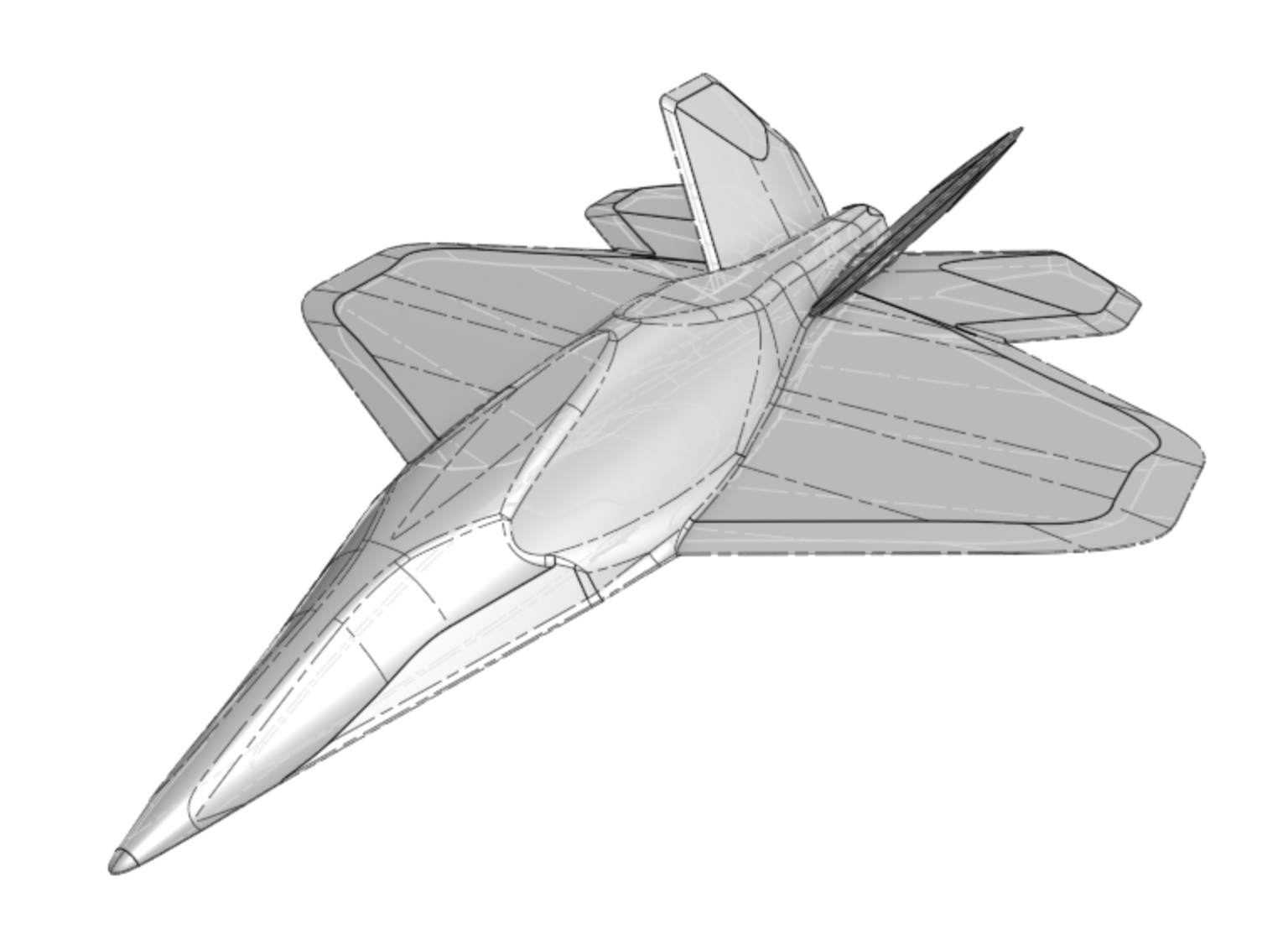CAD of Vehicle Body

To create the curves which represent the 3D structure of the body, I extrude a surface through the part which crosses the entirety of the shape, snaking back and forth at each turn. This was done to simplify the number of objects in the model. The curves will all lie on parallel planes with equal spacing between each. The planes are oriented at a diagonal to the vehicle to accentuate its dynamic nature (it looks cool).

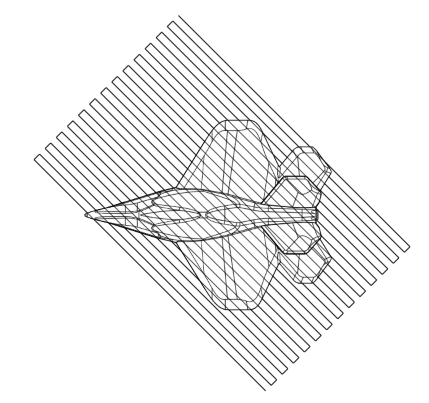Intersection Curve Geometry

Next the surface curves are calculated using the intersection feature applied to the surface and the body.

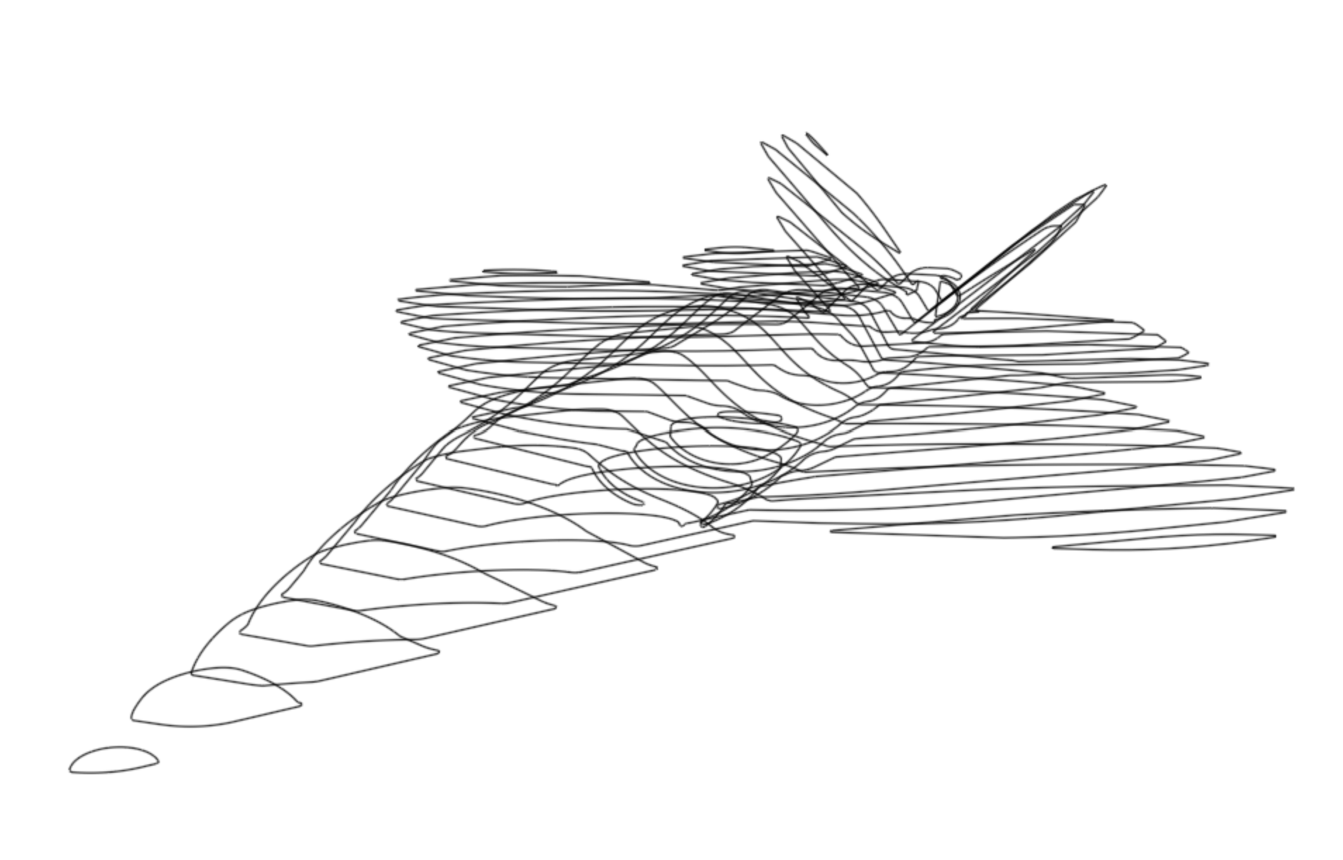Intersection Curves for Render

Okay, this looks cool. But I want to make it fly! To simulate the vehicle motion, I could code up something in MATLAB or C. To plot it in either case, I need the discrete points which describe the curves. Well, if I was working in NX or Solidworks this would be simple. Unfortunately for them, there’s no way I’m paying for CAD software. I could do it in Fusion with a Python script, but I’m already this far in Onshape and I heard you could make custom features with code. How hard could it be?

Coding process condensed for your viewing pleasure

Onshape allows you to create custom features using their language called Featurescript, which is kind of like Java but I have never coded in Javascript so don’t trust me on that. I can say that it was painful to learn, so maybe that’s similar to Java. Anyways, in your Onshape document you can create a new “Feature Studio” where you write up the script which executes your feature. Then you can go into one of the Part Studios and add the feature to your existing geometry.

Instead of starting from scratch, I did some research on Featurescript examples. Turns out Greg Brown at Onshape had solved a similar issue, extracting multiple points from a curve or line. Here is the link to his feature.

This works well for dividing up a single edge into multiple points, but there is a problem with my intersection geometry. Each intersection section is composed of many edges. When I use the tool, I would have to apply the point extraction to each edge individually. This is overbearingly tedious and makes creating evenly spaced points challenging.

To overcome this, I needed to create a feature which allows the user to select multiple adjacent edges which compose a whole curve, then divide up the total length of all segments evenly. Selecting multiple curves is simple, but they are not necessarily in the correct order when selected using a rectangle-drag group selection. The following image demonstrates the issue. When creating the feature, I select all the edges of the curve by dragging a selection rectangle over the entire curve. The component selection menu then lists all the edges selected, however the order is not arranged according to any logic I can identify. In the image I have started at the top of the list and began deleting edges in order. As can be seen by the deselected edges, there is no indication of ordering built into the selection process.

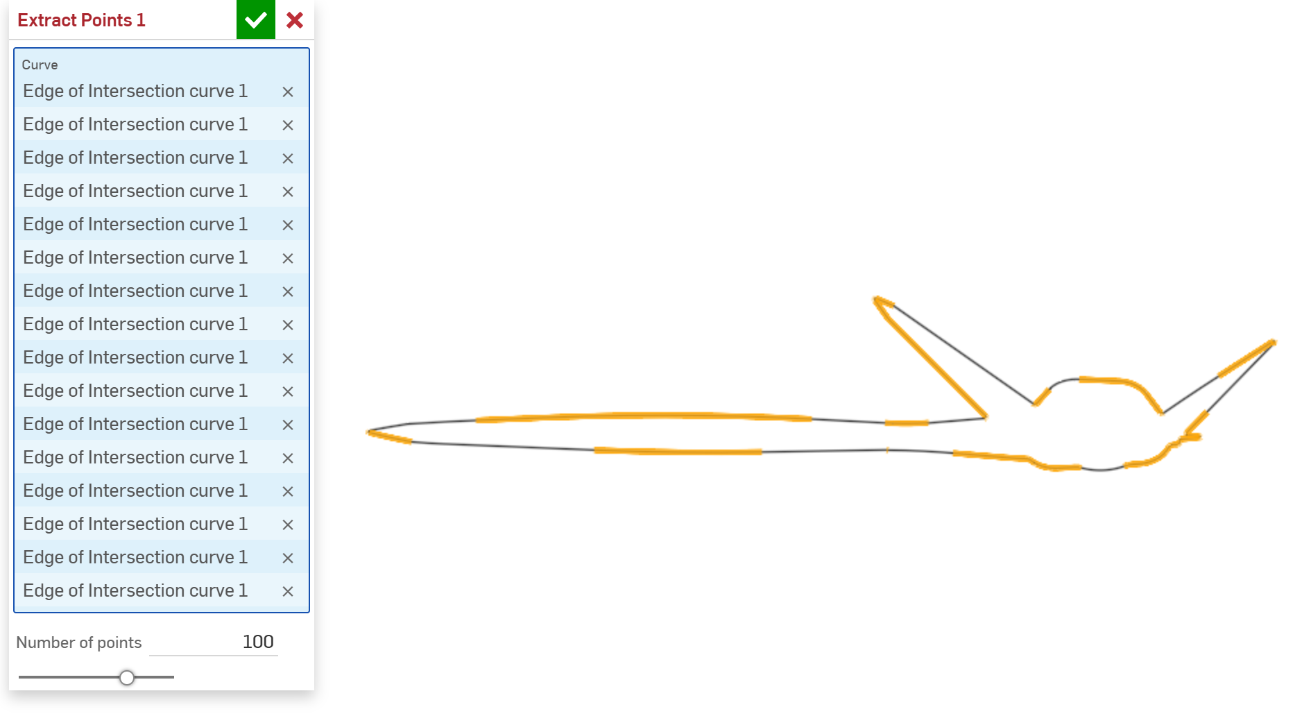Edge Selection for a Complex Curve

Maybe there’s a way to select the whole curve as one object, but I wasn’t able to find it and there’s no way I’m going to click each edge in order. Instead, I coded up a simple sorting algorithm which would start at an arbitrary “first” edge and travel in one direction around the curve, identifying the adjacent curves in order. By requiring that the curve is closed, the sorting process completes by reaching the starting point on the first edge. The search is just basic O(n^2) since it looks through the list of curves on each iteration for the next curve.

Next, since the traversal of each edge is parametrized by a single value that goes from zero to one, determining the orientation of each line described by the parameter relative to its neighbors is important. This requires going through the sorted list of lines and determining which of the two edges was used to match to the previous.

With all the curves in sorted order and orientation tracked, points can now be added according to the even spacing distance. To place the points, all the curves are iterated through once. As the curves are traversed, points are placed according to how much length is available on the current curve after the previously placed point. Any remainder is carried over to the next curve. The point entities are all stored in an array.

Now that I have all the points in an array, the script can just write their coordinates to the custom table structure created by Greg.

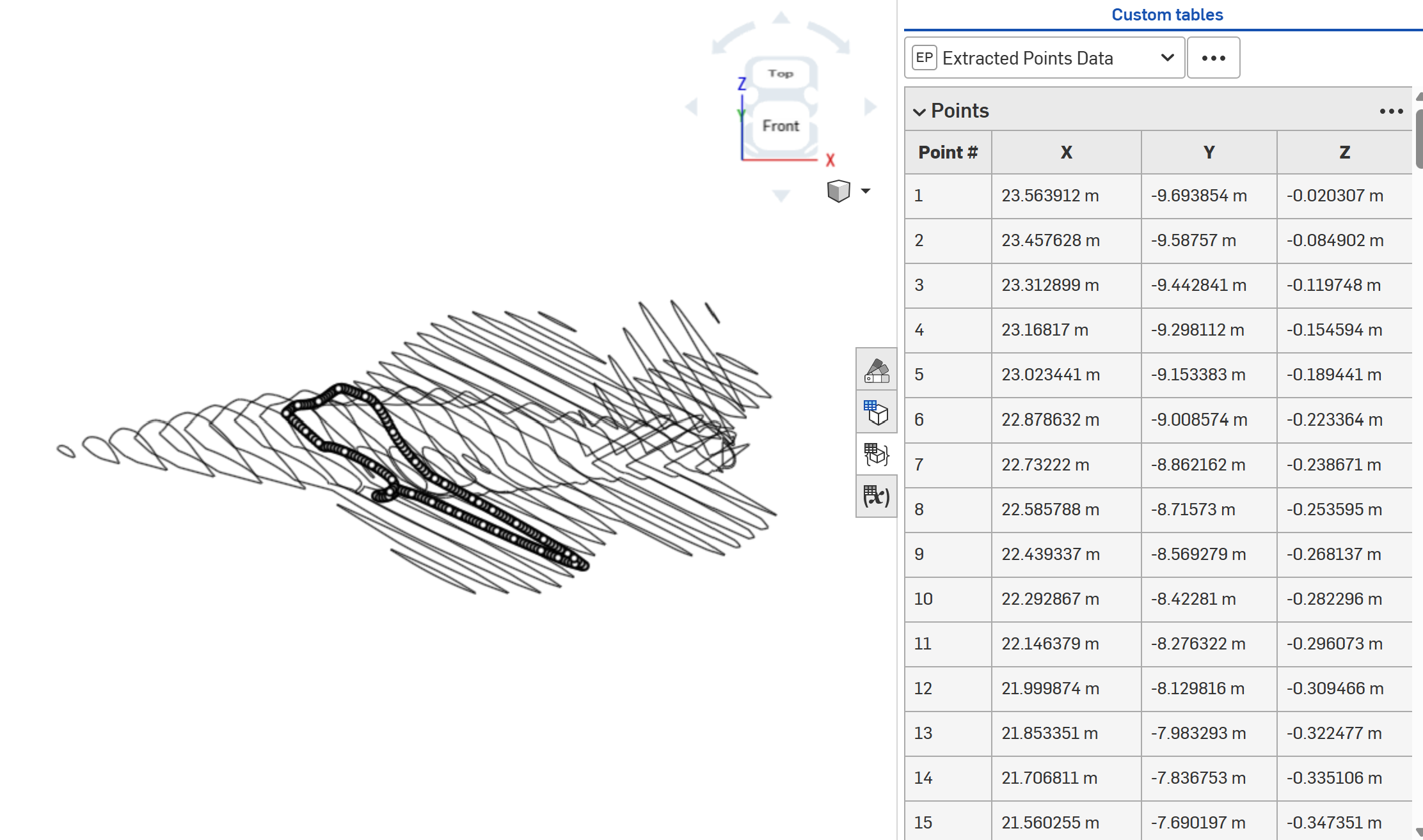Extracted Points

With this feature in place, the process of extracting the point data for a single curve involves adding an Extract Points feature in the CAD features list, selecting all the edges on the curve, specifying the number of points to create, and copying the data from the custom table to a csv or Excel sheet. Now, if I had hundreds of curves, I would need to automate this process; With only 40 curves to do, it’s faster to just crank through them.

This is the link to my Onshape document including my custom Featurescript. Hope you enjoy!

Plotting in MATLAB

Alright, now I have all the data points! What to do with them? Well, I’ll plot them in MATLAB because I’m most familiar with the language. First, since I have all the curves in separate sheets of an excel file, I’ll convert the point data into a data structure which makes sense.

%% Load Excel
sheet_names = sheetnames("plane_coords.xlsx");
n_curves = length(sheet_names);
raw_data = cell(n_curves,1);
for i = 1:n_curves
    raw_data{i} = readcell("plane_coords.xlsx",'Sheet',sheet_names(i));
end

%% Convert Point Data to Correct Format
point_data = cell(n_curves,1);
for i = 1:n_curves
    sel_data = raw_data{i};
    n_points = size(sel_data,1) - 1;
    curve_data = zeros(n_points,3);
    for j = 1:n_points
        for col = 2:4
            pos_string = sel_data{j+1,col};
            num_string = erase(pos_string,' m');
            curve_data(j,col-1) = str2double(num_string);
        end
    end
    point_data{i} = curve_data;
end

%% Save Point Data
save("point_data.mat","point_data")

Alright, now we can plot the data, make it pretty, and animate the gif. The script is below. It is pretty well commented, so feel free to follow along for yourself. Thanks for reading this article!

%==========================================================================
%% Render Plane with Watermark
% // Description:
% Render plane animation but include a signature watermark in the
% background.
%==========================================================================
% // Author: Calder Leppitsch
% // DISCLAIMER: This project is a personal project developed by me outside
% of my work for any employer. It was created entirely using my own
% equipment and resources, and is not affiliated with or endorsed by any
% company. In no way does it make use of company property, intellectual or
% otherwise.
% // Update Log:
% |    Version    |     Date     |     Description
% |      2.0      |  06/24/2025  | Updated the program to include a
%                                   signature watermark in the background
% |      2.1      |  11/08/2025  | Added extra comments for website

clc
clear
close all

%% // Begin Script
% Load point data from Onshape extracted points
load("point_data.mat")

% Number of slices in the plane rendering graphic
n_curves = length(point_data);

% // Create gradation for color-changing effect
% Load the color scheme
CS = loadColor("CH");
% Number of colors in color scheme
n_cs = length(CS);
% Number of subdivisions per color in the color scheme
n_grad_subdiv = 15;
% Subdivide colors and store color values in cell structure
c_holder = cell(n_cs-1,1);
for i = 1:n_cs-1
    c_holder{i} = gradation(hex2rgb(CS(i)),hex2rgb(CS(i+1)),n_grad_subdiv);
end
% Transform color values into array
c_list1 = cat(1,c_holder{:});
% Get full number of colors in gradient array
num_colors = size(c_list1,1);
% Create looping color scheme by appending flipped array
c_list2 = cat(1,c_list1,flip(c_list1,1));

%% // Create color map for encoding to GIF
bg_color = [1, 1, 1]; % Background color to use for transparency
% Create color map for GIF. Encoding holds up to 256 values.
cmap = [c_list1; repmat(c_list1(end,:), 256 - num_colors, 1)];
% Make the last entry the background color
cmap(end,:) = bg_color;
% Keep the background color index for later use. Note subtract one because
% the gif encoding format starts with index 0.
bg_index = 256 - 1;
% Add watermark color and include in color map
watermark_color = [45, 45, 45]/255;
cmap(end-1,:) = watermark_color;

% The rotation function I created doesn't work correctly for points with a
% zero z-coordinate, so need to offset them by a small amount.
% Store point data
point_data_raw = point_data;
% Overwrite point data variable
point_data = cell(n_curves,1);
for i = 1:n_curves
    point_data_sel = point_data_raw{i};
    % Change all zero z values to a small non-zero value.
    point_data_sel(point_data_sel(:,3) == 0,3) = 1e-5;
    point_data{i} = point_data_sel;
end

% // Plot the data and format for rendering
plane_fig = figure;
plane_ax1 = axes('Parent',plane_fig);
plot3(NaN,NaN,NaN)
hold on
% Create cell array for holding the plotted line objects
P = cell(n_curves,1);
for i = 1:n_curves
    curve = point_data{i};
    x = curve(:,1); y = curve(:,2); z = curve(:,3);
    % Initialize plotted line object
    P{i} = plot3(x,y,z,'LineWidth',1,'LineStyle','-.','Color',CS(1));
end
% Set limits for plot based on length of vehicle.
render_cube_sl = 35;
xlim([0 render_cube_sl])
ylim([-render_cube_sl/2,render_cube_sl/2])
zlim([-render_cube_sl/2,render_cube_sl/2])

% Get screen size for plotting in the center of the screen
screen = get(0,'screensize');
% Set render side length dimension in pixels. 
render_pixel_sl = 1000;
plot_dims = [render_pixel_sl render_pixel_sl];
% Place render in center of screen
centerScreen = [0.5*(screen(3)-plot_dims(1)) 0.5*(screen(4)-plot_dims(2)) plot_dims(1) plot_dims(2)];
blScreen = [0 0 render_pixel_sl render_pixel_sl];
% Set background color to the desired value
set(plane_fig, 'Position', blScreen, 'color', bg_color, ...
    'MenuBar', 'none', 'ToolBar', 'none', 'NumberTitle', 'off')
% Set axes size
set(plane_ax1,'Position',[0 0 1 1])
axPos = getpixelposition(plane_ax1);
% No axes, no grid
axis off
grid off
shading interp
% Viewing position vector
view([-1 0 0.2])
% Aspect ratio for viewpoint to get accurate perspective
daspect([1 1 1])

%% // Render Watermark
% Get axes frame size in pixels
ax2 = axes('Position', plane_ax1.Position);
% Move background axes to back
uistack(ax2, 'bottom');

% Load watermark picture
[wmk.img, ~, wmk.alpha] = imread('CJJL_w.png');
% Convert to float
wmk.img = im2double(wmk.img);
wmk.alpha = im2double(wmk.alpha);
[wmk.h, wmk.w] = size(wmk.alpha);
% Add padding to make the image smaller
wmk.img_lg = zeros(3*wmk.h,3*wmk.w,3,'double');
inset_h_ind = (wmk.h+1):(2*wmk.h);
inset_w_ind = (wmk.w+1):(2*wmk.w);
wmk.img_lg(inset_h_ind,inset_w_ind,:) = wmk.img;
% Resize image to frame
wmk.img_resize = imresize(wmk.img_lg, [render_pixel_sl render_pixel_sl], 'nearest');
% Replace all white with watermark color. If not perfectly white, replace
% with white for background color.
for h_lcv = 1:render_pixel_sl
    for w_lcv = 1:render_pixel_sl
        if wmk.img_resize(h_lcv,w_lcv,1) == 1
            wmk.img_resize(h_lcv,w_lcv,:) = watermark_color;
        else
            wmk.img_resize(h_lcv,w_lcv,:) = 1;
        end
    end
end

% Show the image in the background
hImg = imshow(wmk.img_resize, 'Parent', ax2);
set(hImg, 'Interpolation', 'nearest');

%% Create GIF
% Filename
gif_filename = 'calderplane1.gif';
% Frames per second for the gif. Upper limit = ?
fps = 30;

% Time parameters for animation
t_i = 0;
t_s = 1/fps;
t_f = 2*num_colors*t_s;
time = t_i:t_s:t_f;
n_ts = length(time);

% Center point for rotation
rot_pt = [16 0 0];
% Vector representative of axis of rotation emanating from rotation center
% point
rot_ax = [0 0 1];
% Rotation limits (deg)
theta_i = 0; % If this is not zero, then the data used for plot 
% intialization must change
theta_f = 360; % To maintain continuity of the looping gif it should
% complete a full rotation
theta = linspace(theta_i,theta_f,n_ts);

% Capture frame
frame = getframe(plane_fig);
im = frame2im(frame);
im_ind = rgb2ind(im, cmap); % Convert frame using fixed colormap
% Write first frame to gif
imwrite(im_ind, cmap, gif_filename, 'gif', 'LoopCount', Inf, 'DelayTime', t_s, 'TransparentColor', bg_index);

% Loop for the remaining timesteps
for i = 2:n_ts
    c_theta = theta(i);
    % Rotate all curves
    for j = 1:n_curves
        curve = point_data{j};
        curve_rotated = rotate_points(curve,c_theta,rot_pt,rot_ax);
        P{j}.XData = curve_rotated(:,1);
        P{j}.YData = curve_rotated(:,2);
        P{j}.ZData = curve_rotated(:,3);
        P{j}.Color = c_list2(mod(i,num_colors*2)+1,:);
    end
    drawnow
    pause(t_s)

    % Capture frame
    frame = getframe(plane_fig);
    im = frame2im(frame);
    im_ind = rgb2ind(im, cmap); % Convert frame using fixed colormap

    % Write frame to GIF with transparency
    imwrite(im_ind, cmap, gif_filename, 'gif', 'WriteMode', 'append', 'DelayTime', t_s, 'TransparentColor', bg_index, 'DisposalMethod', 'restoreBG');
end
close(plane_fig)

Final Render